讀書筆記：《用Google玩人工智慧實驗》

若您覺得文章寫得不錯，請點選文章上的廣告，來支持小編，謝謝。

If you like this post, please click the ads on the blog or buy me a coffee. Thank you very much.

最近幾年資訊科技一直圍繞在人工智慧與物聯網(物廉網)上，而《用Google玩人工智慧實驗》這本書介紹了只需開起瀏覽器就可以在電腦、手機、平板上體驗人工智慧實驗，於是筆者就高興地閱讀此書了。

第1章 認識人工智慧

此章介紹了人工智慧的定義與起源，以及它的發展與現況。在1956年，科學家在一次的研討會中，提出「人工智慧」一詞，希望機器能夠使用語言、能理解抽象概念、能解決只有人類可解決的問題、能自我改良等。而Alan Turing提出了 Turing Test來檢驗機器是否具有智慧。

人工智慧經歷過幾次的起伏，從「推理與探索」到「專家系統」到「深度學習」為主流的精采歷史。目前人工智慧可大約分成專用型人工智慧(弱人工智慧)以及通用型人工智慧(強人工智慧)兩種。

世界各大企業持續提供方便的人工智慧工具，例如Google AI Experiments。

第2章人工智慧如何運作
此章介紹了人工智慧如何運作以及機器學習、類神經網路、深度學習的基礎觀念。機器學習、類神經網路、深度學習的關係可參考下圖：

人工智慧研究如何讓機器(電腦)表現得有智慧，於是得先有資料給它進行學習(輸入)，讓電腦進一步計算與分析(處理)，最後產生結果或功能(輸出)，如下圖所示：

機器學習通常分為三種類型：監督式學習(Supervised Learning)、非監督式學習(Unsupervised Learning)、強化學習(Reinforcement Learning)。

深度學習是從類神經網路發展而來的，而類神經網路利用機器來模擬人腦神經系統運作模式。( https://playground.tensorflow.org/ )

類神經網路如下圖所示，含有輸入層(Input Layer)、隱藏層(Hidden Layer)、輸出層(Output Layer)。

圖上的每一個圓圈為一個節點，是模仿生物神經元發送訊號。每個節點的輸出若高於一個指定的臨界值，就會啟動該節點，並將訊號傳送給下一個節點。而深度學習為含有多個隱藏層(通常為三層以上)的類神經網路。

AI Experiments 實作體驗

Teachable Machine 網站：https://teachablemachine.withgoogle.com/

Teachable Machine 教學影片：https://www.youtube.com/watch?v=3BhkeY974Rg

操作說明(後續附上連結)

Tensorflow Playground 網站：https://playground.tensorflow.org/

操作說明(後續附上連結)

第3章人工智慧的影像辨識與應用
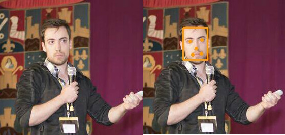
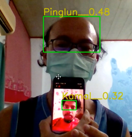
人工智慧影像辨識是研究與展現最多的應用之一，因為視覺很讓人容易感到很多的體驗。

圖像的基本單位為像素，一個像素不見得是正方形，可以是點、線、或是平滑的線。下圖取自 https://en.wikipedia.org/wiki/Pixel。

彩色圖像(Color Image) 大致分為兩種圖像格式：RGB與CMYK。電腦如何處理影像可以參考演算法筆記網站的Image說明。 

機器學習的影像資訊處理過程：原始影像 --> 特徵提取 --> 群集分類 --> 辨識學習 --> 模型應用

資料集

MNIST手寫資料集 http://yann.lecun.com/exdb/mnist/

ImageNet 影像資料集 https://www.image-net.org/

ILSVRC競賽 https://image-net.org/challenges/LSVRC/

影像辨識應用：智慧城市、智慧辦公室、智慧零售、智慧家庭

AI Experiments 實作體驗

Thing Translator 網站：https://experiments.withgoogle.com/thing-translator

操作說明(後續附上連結)

Giorgio Cam 網站：https://experiments.withgoogle.com/giorgio-cam

操作說明(後續附上連結)

Emoji Scavenger Hunt 網站：https://experiments.withgoogle.com/emoji-scavenger

操作說明(後續附上連結)

Move Mirror 網站：https://experiments.withgoogle.com/move-mirror

操作說明(後續附上連結)

AutoDraw 網站：https://experiments.withgoogle.com/autodraw

操作說明(後續附上連結)

Cartoonify 網站：https://experiments.withgoogle.com/cartoonify

操作說明(後續附上連結)

Quick, Draw! 網站：https://experiments.withgoogle.com/quick-draw

操作說明(後續附上連結)

Sketch-RNN Demos 網站：https://experiments.withgoogle.com/sketch-rnn-demo

操作說明(後續附上連結)

Scrying Pen 網站：https://experiments.withgoogle.com/scrying-pen

操作說明(後續附上連結)

Handwriting with a Neural Net 網站：https://experiments.withgoogle.com/handwriting-with-a-neural-net

操作說明(後續附上連結)

第4章人工智慧的聲音、音樂技術與應用
聲音介紹，波動。聲波的振幅、聲波的頻率、聲波的波形。

機器學習的聲音資訊處理過程：原始聲音 --> 特徵提取 --> 群集分類 --> 模型應用

各類聲音辨識競賽

Speech Recognition Low-resource speech recognition with Dynamic Time Warping

TensorFlow Speech Recognition Challenge

AI Experiments 實作體驗

Bird Sounds 網站：https://experiments.withgoogle.com/bird-sounds

操作說明(後續附上連結)

The Infinite Drum Machine 網站：https://experiments.withgoogle.com/drum-machine

操作說明(後續附上連結)

AI Duet 網站：https://experiments.withgoogle.com/ai-duet

操作說明(後續附上連結)

NSynth: Sound Maker 網站：https://experiments.withgoogle.com/sound-maker

操作說明(後續附上連結)

Beat Blender 網站：https://experiments.withgoogle.com/beat-blender

操作說明(後續附上連結)

Melody Mixer 網站：https://experiments.withgoogle.com/melody-mixer

操作說明(後續附上連結)

第5章人工智慧的文字、語言技術與應用

自然語言處理過程：文字或語音資料 --> 字詞分析 --> 語意理解 --> 生成語言 

這看起來好像很輕鬆容易，但對電腦而言這不是很容易，這件事情和符號接地問題(https://en.wikipedia.org/wiki/Symbol_grounding_problem)有關。

聊天機器人「小冰」

AI Experiments 實作體驗

Semantris 網站：https://experiments.withgoogle.com/semantris

操作說明(後續附上連結)

Talk to Books 網站：https://experiments.withgoogle.com/talk-to-books

操作說明(後續附上連結)

Font Map 網站：https://experiments.withgoogle.com/font-map

操作說明(後續附上連結)

Fontjoy 網站：https://experiments.withgoogle.com/fontjoy

操作說明(後續附上連結)

Scribbling Speech 網站：https://experiments.withgoogle.com/scribbling-speech

操作說明(後續附上連結)

第6章人工智慧創意應用
AI和硬體整合(如Arduino、Microbit、ESP32、Raspberry PI等)後，產生了虛擬整合的智慧物聯網(AIoT)。

AI Experiments 實作體驗

Morse + WaveNet Starter Code 網站：https://experiments.withgoogle.com/morse-speak-demo

操作說明(後續附上連結)

Rock-Paper-Scissor Machine 網站：https://experiments.withgoogle.com/rock-paper-scissors

操作說明(後續附上連結)

NSynth Super 網站：https://experiments.withgoogle.com/nsynth-super

操作說明(後續附上連結)

Sound-Controlled Intergalactic Teddy 網站：https://experiments.withgoogle.com/sound-teddy

操作說明(後續附上連結)

Objectifier Spatial Programming 網站：https://experiments.withgoogle.com/objectifier-spatial-programming

Semi-Conductor 網站：https://experiments.withgoogle.com/semi-conductor

操作說明(後續附上連結)

Imaginary Soundcape 網站：https://experiments.withgoogle.com/imaginary-soundscape

操作說明(後續附上連結)

Tree Search: BFS, DFS, Best-First, and A* Search

This example is from MIT OCW Artificial Intelligence.

Consider the tree shown below. The numbers on the arcs are the arc lengths; the numbers

near states B, C, and D are the heuristic estimates; all other states have a heuristic estimate

of 0.

Assume that the children of a node are expanded in alphabetical order when no other order

is specified by the search, and that the goal is state J . No visited or expanded lists are used.

What order would the states be expanded by each type of search. Write only the sequence

of states expanded by each search.

Breadth First

Setep 1:

Visited: A

Queue: B, C, D

Step 2:

Visited: A, B

Queue: C, D, E, F G

Step 3:

Visited: A, B, C

Queue: D, E, F G, H

Step 4:

Visited: A, B, C, D

Queue: E, F, G, H, I, J

Step 5:

Visited: A, B, C, D, E

Queue: F, G, H, I, J

Step 6:

Visited: A, B, C, D, E, F

Queue: G, H, I, J

Step 7:

Visited: A, B, C, D, E, F, G

Queue: H, I, J

Step 8:

Visited: A, B, C, D, E, F, G, H

Queue: I, J

Step 9:

Visited: A, B, C, D, E, F, G, H, I

Queue: J

Step 10:

Visited: A, B, C, D, E, F, G, H, I, J

Queue:

Path for BFS: A, B, C, D, E, F, G, H, I, J

Depth First

Step 1:

Visited: A

Stack: B, C, D

Step 2:

Visited: A, B

Stack: E, F, G, C, D

Step 3:

Visited: A, B, E

Stack: F, G, C, D

Step 4:

Visited: A, B, E, F

Stack: G, C, D

Step 5:

Visited: A, B, E, F, G

Stack: C, D

Step 6:

Visited: A, B, E, F, G, C

Stack: H, D

Step 7:

Visited: A, B, E, F, G, C, H

Stack: D

Step 8:

Visited: A, B, E, F, G, C, H, D

Stack: I, J

Step 9:

Visited: A, B, E, F, G, C, H, D, I

Stack: J

Step 10:

Visited: A, B, E, F, G, C, H, D, I, J

Stack:

Path for DFS: A, B, E, F, G, C, H, D, I, J

Best-First

Node	h(n)
A	0
B	1
C	6
D	3
E	0
F	0
G	0
H	0
I	0
J	0

Step 1:

Open: A

Close:

Step 2:

Open: B, C, D

Close: A

h(B) = 1 ==> the lowest

h(C) = 6

h(D) = 3

Step 3:

Open: C, D, E, F, G

Close: A, B

h(C) = 6

h(D) = 3

h(E) = 0 ==> the lowest

h(F) = 0

h(G) = 0

Step 4:

Open: C, D, F, G

Close: A, B, E

h(C) = 6

h(D) = 3

h(F) = 0 ==> the lowest

h(G) = 0

Step 5:

Open: C, D, G

Close: A, B, E, F

h(C) = 6

h(D) = 3

h(G) = 0 ==> the lowest

Step 6:

Open: C, D,

Close: A, B, E, F, G

h(C) = 6

h(D) = 3 ==> the lowest

Step 7:

Open: C, I, J

Close: A, B, E, F, G, D

h(C) = 6

h(I) = 0 ==> the lowest

h(J) = 0

Step 8:

Open: C, J

Close: A, B, E, F, G, D, I

h(C) = 6

h(J) = 0 ==> the lowest

Step 9:

Open: C

Close: A, B, E, F, G, D, I, J

Reach the Goal J

Path for Best-First: A, B, E, F, G, D, I, J

A*-Search

Node	h(n)
A	0
B	1
C	6
D	3
E	0
F	0
G	0
H	0
I	0
J	0

Step 1:

Open: A

Close:

Step 2:

Open: B, C, D

Close: A

f(A->B) = h(B) + g(A->B) = 1 + 5 = 6 ==> the lowest

f(A->C) = h(C) + g(A->C) = 6 + 2 = 8

f(A->D) = h(D) + g(A->D) = 3 + 4 = 7

Step 3:

Open: C, D, E, F, G

Close: A, B

f(A->B->E) = f(A->B) + h(E) + g(B->E) = 6 + 0 + 6 = 12

f(A->B->F) = f(A->B) + h(F) + g(B->F) = 6 + 0 + 3 = 9

f(A->B->G) = f(A->B) + h(G) + g(B->G) = 6 + 0 + 4 = 10

f(A->C) = h(C) + g(A->C) = 6 + 2 = 8

f(A->D) = h(D) + g(A->D) = 3 + 4 = 7 ==> the lowest

Step 4:

Open: C, E, F, G, I, J

Close: A, B, D

f(A->D->I) = f(A->D) + h(I) + g(D->I) = 7 + 0 + 6 = 13

f(A->D->J) = f(A->D) + h(J) + g(D->J) = 7 + 0 + 3 = 10 ==> the lowest

Step 5:

Open: C, E, F, G, J

Close: A, B, D, J

Reach the Goal J

Path for A*: A, B, D, J

Python 人臉辨識應用「戴不戴口罩」

若您覺得文章寫得不錯，請點選文章上的廣告，來支持小編，謝謝。

If you like this post, please click the ads on the blog or buy me a coffee. Thank you very much.

此文的程式為修改 Github 上的專案：R4j4n/Face-recognition-Using-Facenet-On-Tensorflow-2.X

戴不戴口罩辨識方法

人臉辨識需要經過人臉偵測、特徵擷取、人臉分類(如下圖)來取得某張人臉特徵是誰的人臉。

而常見人臉辨識流程為

1. 使用 mtcnn 偵測人臉特徵如額頭、眼睛、耳朵、鼻子、嘴巴、下巴。

2. 將這些特徵與某人做對應關係。

3. 將多人的人臉特徵使用Facenet做分類訓練。

取得的整張人臉特徵如下圖橘色長方形

戴口罩人臉辨識流程為

1. 使用 mtcnn 偵測人臉的上半部特徵如額頭、眼睛、耳朵、鼻子。

2. 將這些特徵與某人做對應關係。

3. 將多人的人臉特徵使用Facenet做分類訓練。

透過擷取人臉的上半臉如下圖綠色長方形

成果

實作環境Environment

OS:Windows 10

IDE: anaconda Anaconda3-2021.05-Windows-x86_64

到 https://www.anaconda.com/products/individual#Downloads 下載最新版本。

函數庫(Libraries)安裝:

安裝tensorflow 2.3.0

可參考 TensorFlow — Anaconda documentation

無GPU安裝

conda create -n tf tensorflow

conda activate tf

有GPU安裝

conda create -n tf-gpu tensorflow-gpu

conda activate tf-gpu

安裝 Python Package

pip install numpy

pip install opencv-python

pip install mtcnn

pip install scikit-learn

pip install scipy

 

在 Faces 資料夾下建立B某的資料夾，然後將B某的兩到三張照片放到B某資料夾。注意：Faces 資料夾下的人名請用英文。

執行 train_v2.py 做訓練，執行 detect.py 做人臉辨識。

結果影片：

train_v2.py程式碼：

# architecture 模組，含有 FaceNet 網路架構 InceptionResNetV2
from architecture import * 
# 作業系統常用函式庫，如列出資料夾所有檔案
import os 
# 電腦視覺處理函式庫
import cv2
# Multi-task Cascaded Convolutional Neural Networks
# 用來偵測人臉
import mtcnn
# 讀取與儲存 Python 物件函式庫
import pickle 
# 多維度陣列運算的數學函式庫
import numpy as np
# Normalizer 正規化函式庫
from sklearn.preprocessing import Normalizer
# 讀取神經網路模型函式庫
from tensorflow.keras.models import load_model

###### 路徑與變數 ##########
face_data = 'Faces/'

# 將圖片中人臉，做正規化後的大小
required_shape = (160,160)

# facenet 編碼器
face_encoder = InceptionResNetV2()

# 設定 google facenet 建立好的模型參數檔案路徑 
path = "facenet_keras_weights.h5"

# 讀取 google facenet 的模型參數
face_encoder.load_weights(path)
# 使用 mtcnn 人臉偵測器
face_detector = mtcnn.MTCNN()

# 訓練後的人臉編碼串列
encodes = []
# 訓練後的人臉編碼表
encoding_dict = dict()

# L2 正規化
l2_normalizer = Normalizer('l2')

###############################
# 正規化
def normalize(img):
    mean, std = img.mean(), img.std()
    return (img - mean) / std


# 對 Faces 資料夾下的每一人，擷取臉部特徵
for face_names in os.listdir(face_data):
    
    # 設定某甲的人臉資料夾路徑
    person_dir = os.path.join(face_data,face_names)

    # 讀取某甲的每一張臉
    for image_name in os.listdir(person_dir):
        # 設定某甲某張臉的檔案路徑
        image_path = os.path.join(person_dir,image_name)

        # 讀取某甲某張臉，BGR的格式
        img_BGR = cv2.imread(image_path)
        # 某甲某張臉 BGR 格式轉換成 RGB 格式，RGB格式才能給 mtcnn 人臉偵測器使用
        img_RGB = cv2.cvtColor(img_BGR, cv2.COLOR_BGR2RGB)

        # 找人臉特徵的位置
        x = face_detector.detect_faces(img_RGB)
        # 框出來的人臉位置長方形 box：x1、y1、width寬、height高
        x1, y1, width, height = x[0]['box']
        
        
        #print(type(height))
        #print(height)
        
        # 將人臉的高度除2，也就是取上半臉
        height = int(height / 2)
        #print(height)
        
        # 框出來的人臉位置長方形 box的左上角位置
        x1, y1 = abs(x1) , abs(y1)
        # 框出來的人臉位置長方形 box的右上角位置
        x2, y2 = x1+width , y1+height
        
        # 從圖片取出人臉
        face = img_RGB[y1:y2 , x1:x2]
        
        # 正規化，讓每一人臉照片的大小都一樣
        face = normalize(face)
        face = cv2.resize(face, required_shape)
        
        # 改變 face 的維度
        face_d = np.expand_dims(face, axis=0)
        # 做預測的編碼
        encode = face_encoder.predict(face_d)[0]
        # 將此張人臉編碼，加到人臉編碼串列
        encodes.append(encode)

    # 將新的人臉編碼加入人臉編碼表
    if encodes:
        encode = np.sum(encodes, axis=0 )
        encode = l2_normalizer.transform(np.expand_dims(encode, axis=0))[0]
        encoding_dict[face_names] = encode

# 存檔    
path = 'encodings/encodings.pkl'
with open(path, 'wb') as file:
    pickle.dump(encoding_dict, file)

detect.py 程式碼：

# 電腦視覺處理函式庫
import cv2 
# 多維度陣列運算的數學函式庫
import numpy as np
# Multi-task Cascaded Convolutional Neural Networks
# 用來偵測人臉
import mtcnn
# architecture 模組，含有 FaceNet 網路架構 InceptionResNetV2
from architecture import *
# 使用 train_v2 normalize 與 l2_normalizer
from train_v2 import normalize,l2_normalizer
# 使用 cosine 來計算某兩張臉的相似度
from scipy.spatial.distance import cosine
# 讀取神經網路模型函式庫
from tensorflow.keras.models import load_model
# 讀取與儲存 Python 物件函式庫
import pickle

# 偵測到人臉的可信度最低值
confidence_t=0.99
# 相似程度
recognition_t=0.5
# 將圖片中人臉，做正規化後的大小
required_size = (160,160)

# 取得圖片中的人臉 face，人臉位置左上角(x1,y1)與右下角(x2,y2)
def get_face(img, box):
    x1, y1, width, height = box
    x1, y1 = abs(x1), abs(y1)

    # 取上半臉
    height = int(height/2)

    x2, y2 = x1 + width, y1 + height
    face = img[y1:y2, x1:x2]
    return face, (x1, y1), (x2, y2)

# 取得人臉特徵編碼
def get_encode(face_encoder, face, size):
    face = normalize(face)
    face = cv2.resize(face, size)
    encode = face_encoder.predict(np.expand_dims(face, axis=0))[0]
    return encode

# 讀取人臉特徵編碼表
def load_pickle(path):
    with open(path, 'rb') as f:
        encoding_dict = pickle.load(f)
    return encoding_dict

# 偵測人臉
def detect(img ,detector,encoder,encoding_dict):
    # 人臉 BGR 格式轉換成 RGB 格式，RGB格式才能給 mtcnn 人臉偵測器使用
    img_rgb = cv2.cvtColor(img, cv2.COLOR_BGR2RGB)
    # 人臉偵測結果，可能會有好幾處偵測到人臉
    results = detector.detect_faces(img_rgb)
    
    # 對影像中每一處可能為人臉的地方
    for res in results:
        # 此人臉是否有超過 confidence_t ，若沒有超過 0.99，就跳過此人臉
        if res['confidence'] < confidence_t:
            continue

        # 取得圖片中的人臉 face，人臉位置左上角 pt_1 與右下角 pt_2
        face, pt_1, pt_2 = get_face(img_rgb, res['box'])
        # 取得人臉特徵編碼      
        encode = get_encode(encoder, face, required_size)
        # 人臉特徵編碼正規化
        encode = l2_normalizer.transform(encode.reshape(1, -1))[0]
        # 是誰呢？
        name = 'unknown'

        # 與誰的臉最相似
        distance = float("inf")
        
        # 找出與 Faces資料夾下的某人最相似
        for db_name, db_encode in encoding_dict.items():
            # 此人臉與某甲的相似度
            dist = cosine(db_encode, encode)
            # 若有比 recognition_t 0.5 還小，此人臉就非常有可能是這位某甲
            if dist < recognition_t and dist < distance:
                # 將人臉名稱為某甲的姓名
                name = db_name
                # 更新相似度，繼續找更相似的某甲
                distance = dist

        # 將人臉的名稱顯示在圖片上
        if name == 'unknown':
            cv2.rectangle(img, pt_1, pt_2, (0, 0, 255), 2)
            cv2.putText(img, name, pt_1, cv2.FONT_HERSHEY_SIMPLEX, 1, (0, 0, 255), 1)
        else:
            cv2.rectangle(img, pt_1, pt_2, (0, 255, 0), 2)
            cv2.putText(img, name + f'__{distance:.2f}', (pt_1[0], pt_1[1] - 5), cv2.FONT_HERSHEY_SIMPLEX, 1,
                        (0, 200, 200), 2)
    
    # 回傳處理過的圖片，讓更新過的圖片顯示在視訊鏡頭視窗畫面上
    return img 



if __name__ == "__main__":
    # 將圖片中人臉，做正規化後的大小
    required_shape = (160,160)
    # facenet 編碼器
    face_encoder = InceptionResNetV2()
    # 設定 google facenet 建立好的模型參數檔案路徑 
    path_m = "facenet_keras_weights.h5"
    # 讀取 google facenet 的模型參數
    face_encoder.load_weights(path_m)
    # 訓練後的人臉編碼表檔案路徑
    encodings_path = 'encodings/encodings.pkl'
    # 使用 mtcnn 人臉偵測器    
    face_detector = mtcnn.MTCNN()
    
    # 讀取訓練後的人臉編碼表
    encoding_dict = load_pickle(encodings_path)
    
    # 設定鏡頭為作業系統編號0的視訊鏡頭
    cap = cv2.VideoCapture(0)

    # 當成公開啟視訊鏡頭
    while cap.isOpened():
        # 讀取視訊鏡頭影像，ret 為讀取影像的結果狀態，frame為影像本身。
        ret,frame = cap.read()
        # 將影像左右翻轉
        frame = cv2.flip(frame,1)
        
        # 讀取影像沒有成功
        if not ret:
            print("CAM NOT OPEND") 
            break
        
        # 將視訊影像做人臉偵測，並將偵測結果更新到 frame 影像上
        frame = detect(frame , face_detector , face_encoder , encoding_dict)

        # 將人臉偵測結果顯示在式窗上
        cv2.imshow('camera', frame)

        # 若按下按鍵 q，退出程式
        if cv2.waitKey(1) & 0xFF == ord('q'):
            # 釋放視訊鏡頭資源
            cap.release()
            # 關閉程式所開啟的視窗
            cv2.destroyAllWindows()
            break